Up and Running with Metal, Part 3: Lighting and Rendering in 3D

In this post, we’ll finally start rendering in 3D. In order to get there, we’ll talk about how to load 3D model data from disk, how to tell Metal to draw from a vertex buffer using indices, and how to manipulate objects in real time.

This post assumes that you know a little linear algebra. I have written an incomplete introduction to the subject in this post. There are also many excellent resources around the Internet should you need more information on a particular topic.

You can download the sample project for this post here.

Loading OBJ Models

Up until now, we’ve been hardcoding our geometry data directly into the program. This is fine for tiny bits of geometry, but it becomes unsustainable pretty quickly. By storing model data on the file system in a standard format, we can begin to work with much larger datasets.

One of the most popular formats for storing basic 3D model data is the OBJ format. You can read the full specification on Martin Reddy’s site. OBJ files store lists of vertex positions, normals, texture coordinates, and faces in a human-readable format. The sample code includes a rudimentary OBJ parser that can load OBJ models into memory in a suitable format for rendering with Metal. I will not describe the loader in detail here.

The model we use in this post is a teapot. The teapot shape is one of the most recognizable datasets from the early days of computer graphics. It was originally modeled after a Melitta teapot by Martin Newell at the University of Utah in 1975. It frequently makes appearances in graphics tutorials because of its interesting topology and asymmetry.

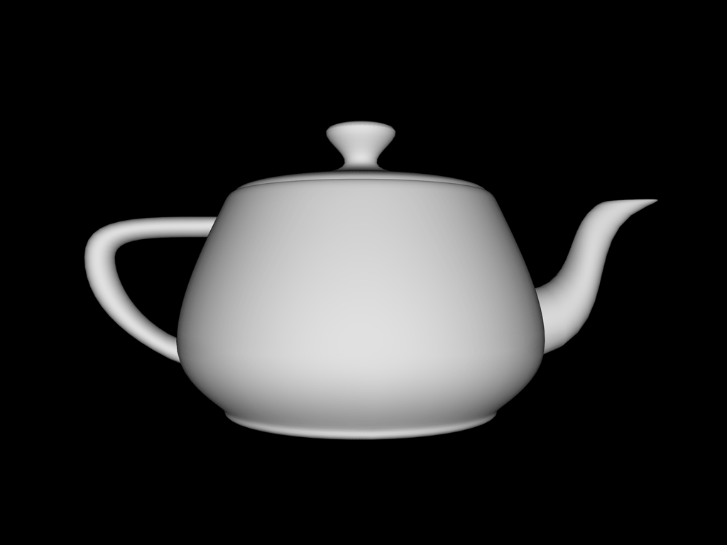
You should feel free to recompile the sample project, replacing the included model with your own OBJ file. Models that are normalized to fit in a 1x1x1 cube around the origin will be the easiest to work with.

Models in OBJ format are logically divided into groups, which are essentially named lists of polygons. Loading a model is as simple as finding the OBJ file in the app bundle, initializing an OBJModel object, and asking for a group by index.

NSURL *modelURL = [[NSBundle mainBundle] URLForResource:@"teapot" withExtension:@"obj"];
OBJModel *teapot = [[OBJModel alloc] initWithContentsOfURL:modelURL];
OBJGroup *group = [teapot groupAtIndex:1];

Index 1 corresponds to the first group in the file; polygons that don’t belong to any group are added to an implicit, unnamed group at index 0.

OBJGroup is a struct with two pointer members: vertices and indices. We’ll see shortly how to put them into buffers and draw them with Metal.

Lighting

In order to start constructing realistic scenes, we need a way to model how light interacts with surfaces. Fortunately, much of computer graphics concerns itself with figuring out clever ways to approximate the behavior of light. We will use an approximation consisting of three terms to model different species of light that occur in a scene: ambient, diffuse, and specular. Each pixel’s color will be the sum of these three terms. Here is the equation representing that relationship at the highest level:

Above, stands for intensity, specifically, outgoing radiant intensity. We’ll use to signify properties of the light source, and to signify properties of the material. None of these values have a precise physical basis. Our first attempt at approximating illumination involves a lot of shortcuts. Therefore, the values we choose for these quantities will be based on aesthetics rather than physical exactitude.

The types of lights we will be dealing with are directional; they do not have a defined position in space. Instead, we imagine that they are far enough away to be characterized exclusively by the direction in which they emit light. The sun is an example of such a directional light.

Ambient Light

Ambient light is a non-directional kind of light that is not associated with a particular light source. Instead, it is an approximation used to model indirect light (light that has bounced off other surfaces in the scene), which is not captured by the other terms. Ambient lighting prevents the parts of geometry that are not directly lit from being completely black. The contribution of ambient light is normally subtle.

Ambient light is calculated as the product of the ambient intensity of the light and the ambient response of the surface:

Usually, the material will have a fairly low ambient response, to represent the fact that ambient light is a minor contribution to the overall reflected intensity.

Diffuse Light

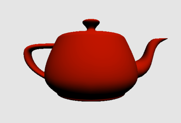
Diffuse light follows Lambert’s cosine law, which states that the intensity of reflected light is directly proportional to the cosine of the angle between the direction of the incident light and the normal of the surface. The normal is a vector that is perpendicular to the surface. Light that is head-on is reflected to a greater degree than light that arrives at a shallow angle of incidence.

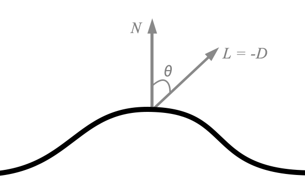
Diffuse reflection is modeled by the following simplified equation:

If we assume that the normal vector and incident light direction vector are unit vectors, we can use the familiar dot product to calculate this term:

Specular Light

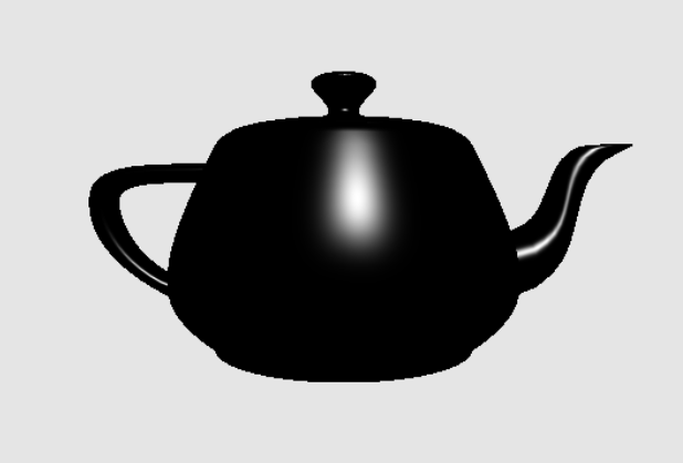
The specular light term is used to model “shiny” surfaces. It models the tendency of the material to reflect light in a particular direction rather than scattering it in all directions. Shiny materials create specular highlights, which are a powerful visual cue for illustrating how rough or shiny surfaces are. “Shininess” is quantified by a parameter called the specular power. For example a specular power of 5 corresponds with a rather matte surface, while a specular power of 50 corresponds to a rather shiny surface.

There are a couple of popular ways to compute the specular term, but here we will use a Blinn-Phong approximation. The Blinn-Phong specular term uses an intermediate vector called the halfway vector that points halfway between the direction to the light source and the direction from which the surface is being viewed:

Once we have the halfway vector in hand, we compute the dot product between the the surface normal and the halfway vector, and raise this quantity to the specular power of the material.

This exponentiation is what controls how “tight” the resulting specular highlights are; the higher the specular power, the sharper the highlights will appear.

The Result

Now that we’ve computed all three terms of our lighting equation, we sum together the results at each pixel to find its final color. In the next few sections, we’ll talk about how to actually achieve this effect with the Metal shading language.

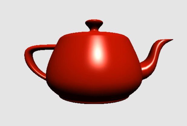
Representing Lights and Materials

We will use two structs to wrap up the properties associated with lights and materials. A light has three color properties, one for each of the light terms we discussed in detail. The ambient color is not actually associated with a particular light, but since we will only be using one light in our sample scene, it makes sense to lump it in with the other properties.

struct Light
{
    float3 direction;
    float3 ambientColor;
    float3 diffuseColor;
    float3 specularColor;
};

A material also has three color properties; these model the response of the material to incoming light. The color of light reflected from a surface is dependent on the color of the surface and the color of the incoming light. As we’ve seen, the color of light and the color of the surface are multiplied together to determine the color of the surface, and this color is then multiplied by some intensity ( in the case of ambient, in the case of diffuse, and raised to some power in the case of specular). We model the specular power as a float.

struct Material
{
    float3 ambientColor;
    float3 diffuseColor;
    float3 specularColor;
    float specularPower;
};

Transforming from 3D to 2D

In order to draw 3D geometry to a 2D screen, the points must undergo a series of transformations: from world space, to eye space, to clip space, through the perspective divide to normalized device coordinates, and finally to screen space.

From Model Space to World Space

Objects are usually modeled around the origin of their local coordinate system. For example, it might make sense for the center of mass of the object to coincide with its coordinate system’s origin. Or, the origin could be another point that is significant to the model, such as a point near the hips of a bipedal model where its skeletal hierarchy is rooted.

In any case, we need a way of positioning the model in a larger universe. This is the purpose of the world transformation, which transforms the points in a model into the coordinate system of the scene in which they reside. The world transformation of a model moves, scales, and rotates it so that it appears correct relative to other objects in the scene.

The world transformation of our teapot will be a sequence of rotations that can be manipulated by the user. When the user pans left or right, the teapot will rotate about its y axis, and when the user pans up and down, the teapot will rotate about its x axis.

The following code shows how we configure the transformation that takes the teapot from model space to world space, by applying these two rotations successively to an identity matrix.

static const simd::float3 X_AXIS = { 1, 0, 0 };
static const simd::float3 Y_AXIS = { 0, 1, 0 };
simd::float4x4 modelMatrix = Identity();
modelMatrix = Rotation(Y_AXIS, -angle.x) * modelMatrix;
modelMatrix = Rotation(X_AXIS, -angle.y) * modelMatrix;

After this sequence of multiplications, modelMatrix is the world transformation.

From World Space to View Space

Now that we have our scene (the rotated teapot) in world space, we need to position the entire scene relative to the eye point of our virtual camera. This transformation is called the view space (or, equivalently, the eye space or camera space) transformation. The position of the virtual camera’s eye is the apex of the viewing volume, the point behind the middle of the near plane of the viewing frustum.

In our sample scene, we will position the camera a little back from the teapot. We do this by directly manipulating the fourth column of the view matrix, which controls the translation of the camera. By setting its z coordinate to a negative number (-1), we move the scene along the negative z axis, which is to say we move the camera along the positive z axis. In our right-handed coordinate system, the positive z axis points out of the screen.

simd::float4x4 viewMatrix = Identity();
viewMatrix.columns[3].z = -1.0;

From View Space to Clip Space

The projection matrix transforms view space coordinates into clip space coordinates. See the article on linear algebra for more details. Metal’s normalized device coordinate (NDC) space is a cuboid , meaning that x and y coordinates range from -1 to 1, and z coordinates range from 0 to 1 as we move away from the camera.

Clip space is the 3D space that is used by the GPU to determine visibility of triangles within the viewing volume. If all three vertices of a triangle are outside the clip volume, the triangle is not rendered at all. On the other hand, if one or more of the vertices is inside the volume, it is clipped to the bounds, and one or more modified triangles are used as the input to the vertex shader.

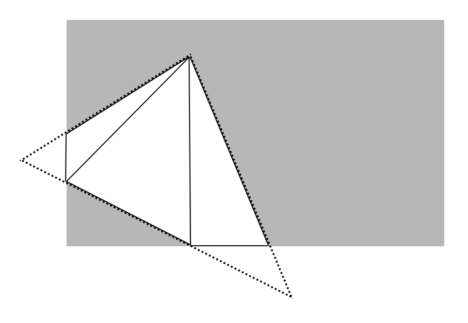
The perspective projection matrix takes points from view space into clip space via a sequence of scaling operations. This is encapsulated in the PerspectiveProjection utility function. We fix a vertical field of view of 75 degrees, choose a far and near plane value, and select an aspect ratio that is equal to the ratio between the current width and height of our Metal view.

const float near = 0.1;
const float far = 100;
const float aspect = self.view.bounds.size.width / self.view.bounds.size.height;
simd::float4x4 projectionMatrix = PerspectiveProjection(aspect, DegToRad(75), near, far);

The resulting projection matrix will be multiplied with the other matrices to produce a few different matrices that we will use in the vertex and fragment shaders.

Projection and Lighting Shaders

We will use the vertex shader primarily to transform points from model space to clip space, and use the fragment shader to do all of our lighting. In order to get the transformation matrices into the shaders, we will use a special structure of uniforms.

Uniforms

A uniform is a value that is passed as a parameter to a shader that does not change over the course of a draw call. From the point of view of a shader, it is a constant.

For convenience, we store the various uniforms we need in one struct:

typedef struct
{
    simd::float4x4 modelViewMatrix;
    simd::float4x4 modelViewProjectionMatrix;
    simd::float3x3 normalMatrix;
} Uniforms;

The model-view matrix is the product of the model and view matrices. As a transformation, takes points directly from model space to view space. The model-view-projection matrix is the product of the model-view and projection matrices. As a transformation, it takes points directly from model space all the way to clip space. This is the most important transformation, since Metal requires positions to be in clip space to do its job.

Finally, the normal matrix is a matrix that transforms surface normals from model space to view space. Vectors transform differently than points, for reasons that are beyond the scope of this article.

We generate a new structure of uniforms each frame, in the -updateUniforms method of our view controller:

Uniforms uniforms;
simd::float4x4 modelView = viewMatrix * modelMatrix;
uniforms.modelViewMatrix = modelView;
simd::float4x4 modelViewProj = projectionMatrix * modelView;
uniforms.modelViewProjectionMatrix = modelViewProj;
simd::float3x3 normalMatrix = { modelView.columns[0].xyz, modelView.columns[1].xyz, modelView.columns[2].xyz };
uniforms.normalMatrix = simd::transpose(simd::inverse(normalMatrix));
self.uniformBuffer = [self.renderer newBufferWithBytes:(void *)&uniforms length:sizeof(Uniforms)];

Uniforms are passed to Metal just like most other data: in a buffer. The -newBufferWithBytes:length: method is a utility on our new renderer class that asks the Metal device to create a new buffer with the default cacheing behavior.

Interleaved Vertex Buffers

It is possible to pass the various properties of our vertices (position, normal, texture coordinates, and so on) in separate buffers, but it is often more convenient to treat the vertex list as an array of tightly-packed structs, each containing the properties of a single vertex.

Using an interleaved format has a couple of benefits. Firstly, we can store all of our vertex data in a single array, and if we want, we can optimize disk storage around our chosen format, which makes streaming data from disk much faster. Secondly, such a layout helps cache coherency by keeping the data that is most likely to be accessed by a shader together in memory. If instead the vertex data is split across multiple buffers, the shader will have to look at several disparate memory locations in order to read the vertex’s various properties.

Vertex Descriptors

In order to tell Metal how we’ve chosen to lay out our vertices in memory, we use an object called a vertex descriptor. A vertex descriptor consists of a series of attributes, each of which tells Metal where a particular vertex property is located in the vertex struct. Here’s our vertex structure:

struct Vertex
{
    simd::float4 position;
    simd::float4 normal;
};

To describe this structure, we use a MTLVertexDescriptor object with two attributes, one for each struct member. We have to explicitly tell Metal how far into the structure each member starts.

MTLVertexDescriptor *vertexDescriptor = [MTLVertexDescriptor vertexDescriptor];
vertexDescriptor.attributes[0].format = MTLVertexFormatFloat4;
vertexDescriptor.attributes[0].bufferIndex = 0;
vertexDescriptor.attributes[0].offset = 0;

vertexDescriptor.attributes[1].format = MTLVertexFormatFloat4;
vertexDescriptor.attributes[1].bufferIndex = 0;
vertexDescriptor.attributes[1].offset = sizeof(float) * 4;

vertexDescriptor.layouts[0].stride = sizeof(float) * 8;
vertexDescriptor.layouts[0].stepFunction = MTLVertexStepFunctionPerVertex;

In this case, since normal follows position, we indicate that the corresponding attribute (at position 1) is sizeof(float) * 4 = 32 bytes from the start of the structure.

We must also provide a stride value which indicates how big the entire structure is, or how far the shader should advance between vertices in the buffer. This is important because we might have a vertex type that is not tightly packed, or the vertex structure could contain other members that are not relevant to the draw calls we will be making.

The vertex descriptor is part of the pipeline state, and is specified by setting the vertexDescriptor property on the render pipeline descriptor from which the pipeline state is created. For this reason, changing the vertex format is an expensive operation, since it requires discarding the pipeline state and building a new one.

Index Buffers

In our previous post on drawing in 2D, we stored the vertices in the order they were to be drawn. This works fine when each vertex will only be drawn once. However, when drawing a closed 3D surface, most vertices will belong to more than one triangle, and duplicating vertices can lead to a lot of waste, especially for large models.

Fortunately, like most graphics libraries, Metal gives us the ability to provide an index buffer along with our vertex buffer. An index buffer is simply a list of indices into the vertex buffer that specifies which vertices make up each triangle.

Creating the Vertex and Index Buffers

The view controller asks the renderer to create buffers for the model data when it loads the OBJ file:

self.vertexBuffer = [self.renderer newBufferWithBytes:group->vertices length:sizeof(Vertex) * baseGroup->vertexCount];
self.indexBuffer = [self.renderer newBufferWithBytes:group->indices length:sizeof(IndexType) * baseGroup->indexCount];

These buffers will be used later when issuing the indexed draw call.

The Vertex Shader

Our vertex shader will take a Vertex, consisting of a position and normal, and return a ProjectedVertex, consisting of the clip-space position, the view-space (eye-space) position, and the view-space normal. The Vertex type is defined to have the same structure as the Vertex type in our Objective-C code, but has annotations added to indicate which structure member maps to each attribute index.

struct Vertex
{
    float4 position [[attribute(0)]];
    float4 normal [[attribute(1)]];
};

struct ProjectedVertex
{
    float4 position [[position]];
    float3 eye;
    float3 normal;
};

The vertex shader itself is straightforward. First, it transforms the position by the model-view-projection matrix to compute the output vertex’s position in clip-space. Then, it computes the view-space position of the vertex by multiplying by the model-view matrix and negating it, thus producing the vector from the camera to the vertex. Finally, it transforms the normal from model space to clip space by multiplying by the normal matrix.

vertex ProjectedVertex vertex_main(Vertex vert [[stage_in]],
                                   constant Uniforms &uniforms [[buffer(1)]])
{
    ProjectedVertex outVert;
    outVert.position = uniforms.modelViewProjectionMatrix * vert.position;
    outVert.eye =  -(uniforms.modelViewMatrix * vert.position).xyz;
    outVert.normal = uniforms.normalMatrix * vert.normal.xyz;

    return outVert;
}

The Perspective Divide

The final part of the transformation from 3D to 2D space is the perspective divide, which happens in between the vertex shader and the pixel shader. This step is done in hardware and is not configurable or programmable. This step divides the x, y, z coordinates of each point by its w coordinate. As part of the construction of the perspective projection transform, the z coordinate of every point becomes equal to 1. The w component is calculated so that the perspective divide produces foreshortening, the phenomenon of farther objects being scaled down more. This division also has the effect of scaling the z coordinate into the unit range [0, 1], which is what is needed for depth comparison.

The Fragment Shader

The fragment shader takes on the work of computing the lighting at each pixel. It is a straightforward implementation based on the lighting theory we discussed earlier:

fragment float4 fragment_main(ProjectedVertex vert [[stage_in]],
                              constant Uniforms &uniforms [[buffer(0)]])
{
    float3 ambientTerm = light.ambientColor * material.ambientColor;

    float3 normal = normalize(vert.normal);
    float diffuseIntensity = saturate(dot(normal, light.direction));
    float3 diffuseTerm = light.diffuseColor * material.diffuseColor * diffuseIntensity;

    float3 specularTerm(0);
    if (diffuseIntensity > 0)
    {
        float3 eyeDirection = normalize(vert.eye);
        float3 halfway = normalize(light.direction + eyeDirection);
        float specularFactor = pow(saturate(dot(normal, halfway)), material.specularPower);
        specularTerm = light.specularColor * material.specularColor * specularFactor;
    }

    return float4(ambientTerm + diffuseTerm + specularTerm, 1);
}

A couple of peculiarities are worth mentioning. First, the halfway vector is chosen by normalizing the sum of the light direction and view direction. This is more numerically stable than computing their average. Second, all of the dot products are wrapped in calls to saturate, which restricts the output to the range [0, 1]. In the case of the diffuse term, a negative dot product indicates that the face is oriented away from the light source, and should not receive any contribution from it.

Drawing

The Renderer Class

Since the sample projects are becoming more complex, it makes sense to take the first step toward a reusable rendering engine, instead of jamming everything into a UIView or UIViewController subclass.

Our renderer will hold the long-lived objects that we use to render with Metal, including things like our device, library, and pipeline state. We will issue commands from the view controller, which will coordinate the loading of assets and maintain reference to the buffers used for drawing.

The renderer is implemented as an Objective-C class and the source code is in Renderer.h/Renderer.m.

Depth and Stencil State

In order to keep objects that are drawn more recently from appearing on top of objects that should appear farther away, we use a data structure called a depth buffer. As each pixel is written into the framebuffer, a fraction between 0 and 1 is written into the depth buffer. This fraction is a logarithmic function of the pixel’s depth between the near and far clipping planes.

The depth comparison function tells Metal what operation it should use to determine if a fragment is eligible to be written to the framebuffer. Here, we will use MTLCompareFunctionLess, which means that a fragment passes the depth test only if its depth value is less than (nearer to the clip plan than) any previous existing fragment at the same x, y position. We also set the depthWriteEnabled flag to indicate that we want the depth value to be stored in the depth buffer for future comparisons.

Since we will not need to configure it as part of our per-frame update, it is created at the same time as the pipeline state and stored as a property on the renderer object.

MTLDepthStencilDescriptor *depthStencilDescriptor = [MTLDepthStencilDescriptor new];
depthStencilDescriptor.depthCompareFunction = MTLCompareFunctionLess;
depthStencilDescriptor.depthWriteEnabled = YES;
self.depthStencilState = [self.device newDepthStencilStateWithDescriptor:depthStencilDescriptor];

We will not be using stencil buffer features in this post.

Preparing the Render Pass and Command Encoder

The renderer class introduces a startFrame method to do all the setup necessary for each frame. The render pass and command encoder are created as before, but some additional configuration is required:

    [self.commandEncoder setDepthStencilState:self.depthStencilState];
    [self.commandEncoder setFrontFacingWinding:MTLWindingCounterClockwise];
    [self.commandEncoder setCullMode:MTLCullModeBack];

The depthStencilState property is set to the previously-configured stencil-depth state object.

The front-face winding order determines whether Metal considers faces with their vertices in clockwise or counterclockwise order to be front-facing. By default, Metal considers clockwise faces to be front-facing. The sample data and sample code prefer counterclockwise, as this makes more sense in a right-handed coordinate system, so this preference is explicitly enforced on the command encoder.

The cull mode determines whether front-facing or back-facing triangles (or neither) should be discarded (“culled”). This is an optimization that prevents triangles that cannot possibly be visible from being drawn.

Issuing the Draw Call

The renderer object sets the necessary buffer properties on the command encoder and then calls the appropriate method to render the vertices.

[self.commandEncoder setVertexBuffer:positionBuffer offset:0 atIndex:0];
[self.commandEncoder setVertexBuffer:uniformBuffer offset:0 atIndex:1];
[self.commandEncoder setFragmentBuffer:uniformBuffer offset:0 atIndex:0];

[self.commandEncoder drawIndexedPrimitives:MTLPrimitiveTypeTriangle
                                indexCount:indexCount
                                 indexType:MTLIndexTypeUInt16
                               indexBuffer:indexBuffer
                         indexBufferOffset:0];

The first parameter (of type MTLPrimitiveType) lets us tell Metal the type of primitive we’ll be rendering, whether points, lines, or triangles. The rest of the parameters tell Metal the count, size, address, and offset of the index buffer to use for indexing into the previously-set position buffer.

Ending the Frame

After the draw call has been made, the renderer will call endEncoding on the command encoder, present the drawable, and commit the command buffer, which is where Metal takes over and draws our geometry into the framebuffer.

Interaction Via Gestures

In order to make the sample app interactive, we will use a gesture recognizer to detect when the user pans the display left, right, up, and down. This will result in the teapot model rotating about its center, around its x and y axes.

The Pan Gesture Recognizer

We will configure a pan gesture recognizer on the Metal view that will report when the user touches down and pans on the screen. Each time the user moves their finger, the gesture recognizer will estimate the velocity of their motion (in screen points per second) and report it. We scale this value down and use it as the angular velocity of the teapot.

- (void)gestureRecognizerDidRecognize:(UIPanGestureRecognizer *)recognizer
{
    CGPoint velocity = [recognizer velocityInView:self.view];
    self.angularVelocity = CGPointMake(velocity.x * kVelocityScale, velocity.y * kVelocityScale);
}

Dynamics

In order to give the interaction more of a physical field, we will add a damping coefficient to the rotation calculation to make the angular velocity degrade over time when the user is not interacting with the model.

Each frame, the previous frame’s time is stored so that the frame duration can be calculated. The angular velocity is then added to the current rotation angles of the teapot, and damped by a constant to slow down the rotation over time:

NSTimeInterval frameTime = CFAbsoluteTimeGetCurrent();
NSTimeInterval frameDuration = frameTime - self.lastFrameTime;
self.lastFrameTime = frameTime;

self.angle = CGPointMake(self.angle.x + self.angularVelocity.x * frameDuration,
                         self.angle.y + self.angularVelocity.y * frameDuration);
self.angularVelocity = CGPointMake(self.angularVelocity.x * (1 - kDamping),
                                   self.angularVelocity.y * (1 - kDamping));

Conclusion

This post covered a lot of ground: loading OBJ models; transformations and projection; per-pixel lighting in the fragment shader; indexed drawing; and user interaction. You should download the sample project here to view the code and explore further.

Future posts will take a look at the use of textures to increase the realism of our rendered images. As always, feel free to leave comments on this post about what you want to see.