Writing a Modern Metal App from Scratch: Part 2

In the previous article, we wrote enough Metal code to get the spinning silhouette of a teapot on the screen, but that still leaves a lot to be desired as far as a “modern” app is concerned. In this article, we’ll further flesh out the app and introduce lighting, materials, texturing, and managing multiple objects with scene graphs.

Remember that you can clone this Github repository to follow along with the sample code.

A Little Bit of Housekeeping

Thanks to some gentle chiding by my pal Greg Heo, I decided to slightly refine the property initialization code in the Renderer class. Rather than use implicitly-unwrapped optionals for members that require long-winded initialization, I refactored the creation of the vertex descriptor and render pipeline state into their own static methods. John Sundell gives a good overview of alternatives here. I find closure-based lazy vars distasteful, so I took the “lightweight factory” approach.

Do a git checkout step2_1 to get a version of the project with the initialization refactorings applied.

And now, back to our regularly-scheduled programming.

Going Deep

Because we’re currently writing a solid color from our fragment function, the 3D nature of the model isn’t really apparent. Let’s make a small modification to the fragment shader so we can visualize the eye-space normal of the model ¹.

fragment float4 fragment_main(VertexOut fragmentIn [[stage_in]]) {
    float3 normal = normalize(fragmentIn.eyeNormal.xyz);
    return float4(abs(normal), 1);
}

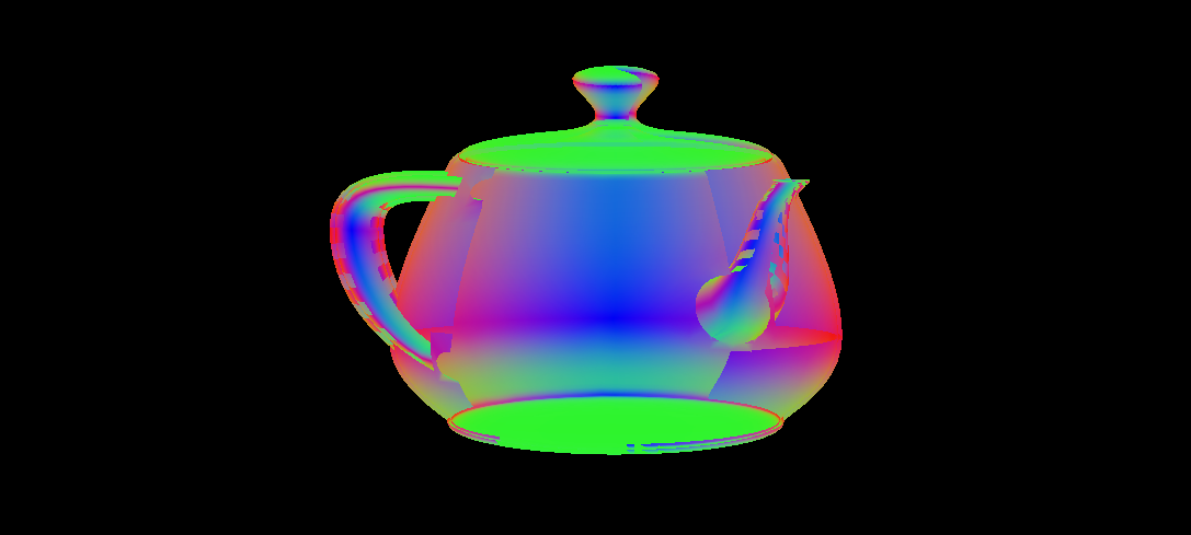
If you run the app now, you’ll notice that portions of the model that shouldn’t be visible are. It’s as though the triangles that comprise the model are being drawn without regard to which should be nearer or farther to the camera. That is, in fact, what is happening. To fix this issue, we need to tell Metal to store the depth of each fragment as we process it, keeping the closest depth value and only replacing it if we see a fragment that is closer to the camera. This is called depth buffering, and fortunately, it’s not too hard to configure.

The Depth Pixel Format

Depth buffering requires the use of an additional texture called, naturally, the depth buffer. This texture is a lot like the color texture we’re already presenting to the screen when we’re done drawing, but instead of storing color, it stores depth, which is basically the distance from the camera to the surface.

First, we need to tell the MTKView which pixel format it should use for the depth buffer. This time, we need to select a depth format, so we choose .depth32Float, which uses one single-precision float per pixel to track the distance from the camera to the nearest fragment seen so far.

Add this to the viewDidLoad() method of the view controller:

mtkView.colorPixelFormat = .bgra8Unorm_srgb
mtkView.depthStencilPixelFormat = .depth32Float

Adding Depth to the Pipeline State

Now the view knows that it needs to create a depth texture for us, but we still need to configure the rest of the pipeline to deal with depth. Specifically, we need to configure our pipeline descriptor with the view’s depth pixel format:

pipelineDescriptor.colorAttachments[0].pixelFormat = view.colorPixelFormat
pipelineDescriptor.depthAttachmentPixelFormat = view.depthStencilPixelFormat

If you were to run the code again at this point, you wouldn’t see any improvement. We still need to tell Metal how to interpret and write to the depth buffer.

The Depth-Stencil State

We do this with a depth-stencil state object. First, add a property to hold a depth-stencil state to the renderer:

let depthStencilState: MTLDepthStencilState

Following the static initializer method approach, we add a method to generate a depth-stencil state:

static func buildDepthStencilState(device: MTLDevice) -> MTLDepthStencilState {
    let depthStencilDescriptor = MTLDepthStencilDescriptor()
    depthStencilDescriptor.depthCompareFunction = .less
    depthStencilDescriptor.isDepthWriteEnabled = true
    return device.makeDepthStencilState(descriptor: depthStencilDescriptor)!
}

The depthCompareFunction is used to determine whether a fragment passes the so-called depth test. In our case, we want to keep the fragment that is closest to the camera for each pixel, so we use a compare function of .less, which replaces the depth value in the depth buffer whenever a fragment closer to the camera is processed.

We also set isDepthWriteEnabled to true, so that the depth values of passing fragments are actually written to the depth buffer. Without this flag set, no writes to the depth buffer would occur, and it would essentially be useless. There are circumstances in which we want to prevent depth buffer writes (such as particle rendering), but for opaque geometry, we almost always want it enabled.

We call our new method in the renderer’s initializer:

depthStencilState = Renderer.buildDepthStencilState(device: device)

Rendering with Depth

Finally, we need to ensure that our render command encoder is actually using our depth-stencil state and our depth buffer to track the depth of each fragment. To do this, we set the depth-stencil state on the render encoder before issuing our draw calls:

commandEncoder.setDepthStencilState(depthStencilState)

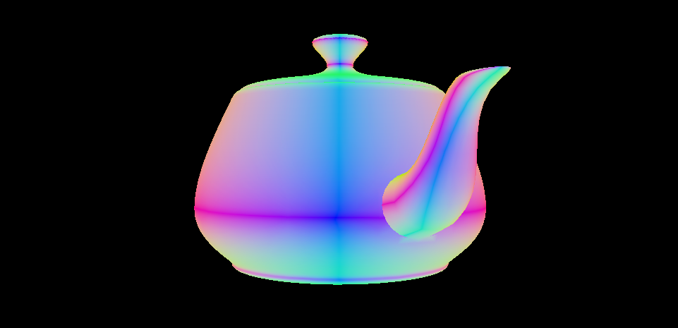
If you run the app after these changes, you should see a much more plausible rendition of the teapot. No more overlapping geometry! (Tea-ometry?)

git checkout step2_2 to view the code up to this point.

Lighting and Materials

The art of illuminating virtual 3D scenes is a deep and much-studied field. We will consider a very basic model here, just enough to create a passable shiny surface. Our basic model calculates the lighting at a particular point as a sum of terms, each of which represents one aspect of how surfaces reflect light. We’ll look at each of these terms in turn: ambient, diffuse, and specular.

Ambient Illumination

The ambient term in our lighting equation accounts for indirect illumination: light that arrives at a surface after it has “bounced” off another surface. Imagine a desk illuminated above by a fluorescent light: even if the light is the only source of illumination around, the floor beneath the desk will still receive some light that has bounced off the walls and floor. Since modeling indirect light is expensive, simplified lighting models such as ours include an ambient term as a “fudge factor,” a hack that makes the scene look more plausible despite being a gross simplification of reality.

To implement ambient illumination in our fragment shader, we declare the “base color” of the object’s material to be bright red, then select an arbitrary “ambient intensity” of 0.3, or 30% of full brightness. The color of the fragment is the product of these two factors as seen in our revised fragment function:

constant float3 ambientIntensity = 0.3;
constant float3 baseColor(1.0, 0, 0);

fragment float4 fragment_main(VertexOut fragmentIn [[stage_in]]) {
    float3 finalColor = ambientIntensity * baseColor;
    return float4(finalColor, 1);
}

For the time being, we lift the definitions of ambient intensity and base color out of the function. We’ll eventually pass them in as uniforms, since we want them to vary from object to object (and maybe from frame to frame).

Ambient illumination produces a flat-looking appearance, since it assumes that indirect light arrives uniformly from all directions.

git checkout step2_3 to view the code up to this point.

Diffuse Illumination

Diffuse illumination represents the portion of light that arrives at a surface and then scatters uniformly in all directions. Think of a concrete surface or a matte wall. These surfaces scatter light instead of reflecting it like a mirror.

Since we thought ahead and already have the surface normal and position in world space² available in our fragment shader, we can compute the diffuse lighting term on a per-pixel basis.

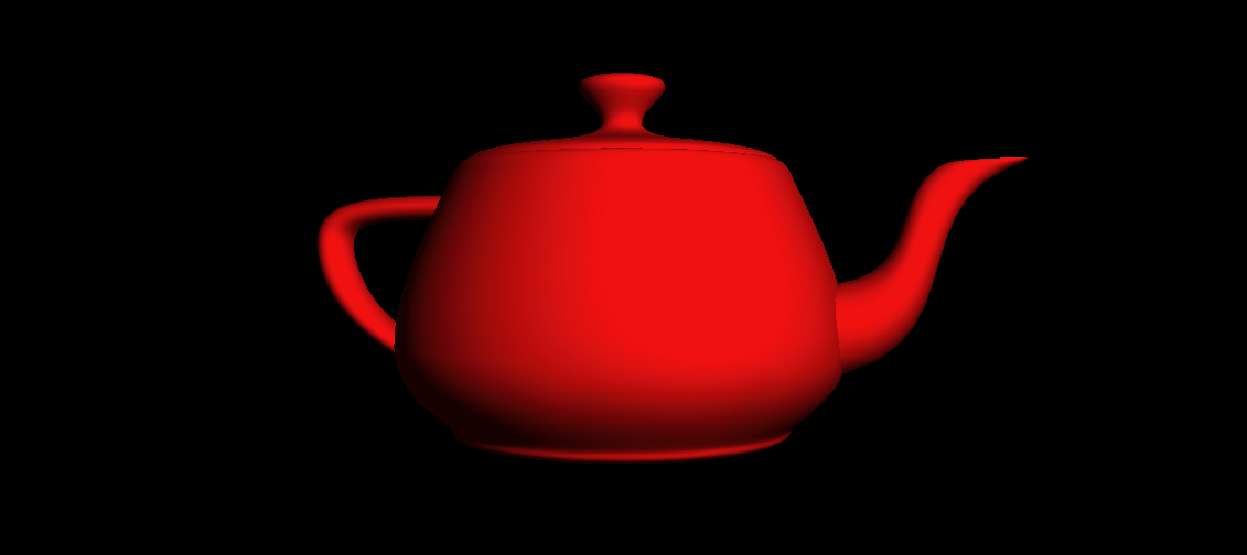
It turns out that there is a fairly simple relation between how much light is reflected diffusely from a surface and its orientation relative to the light source: the diffuse intensity is the dot product of the surface normal (N) and the light direction (L). Intuitively, this means that more light is reflected by a surface that is facing “toward” a light source than one to which the incident light is “glancing.” We can express this by modifying the fragment shader as follows:

constant float3 ambientIntensity = 0.1;
constant float3 lightPosition(2, 2, 2); // Light position in world space
constant float3 lightColor(1, 1, 1);
constant float3 baseColor(1.0, 0, 0);

fragment float4 fragment_main(VertexOut fragmentIn [[stage_in]]) {
    float3 N = normalize(fragmentIn.worldNormal.xyz);
    float3 L = normalize(lightPosition - fragmentIn.worldPosition.xyz);
    float3 diffuseIntensity = saturate(dot(N, L));
    float3 finalColor = saturate(ambientIntensity + diffuseIntensity) * lightColor * baseColor;
    return float4(finalColor, 1);
}

We need to normalize the surface normal in the fragment shader even if each vertex supplies a unit-length normal, because the rasterizer uses linear interpolation to compute the intermediate normal values, which does not preserve length. We calculate the direction to the light, L, as the vector difference between the world-space position of the light and the world-space position of the surface. This vector also needs to be normalized, since it can have arbitrary length.

To compute the diffuse light intensity being reflected from the surface at this point, we take the dot product between N and L, which will be 1 when they are exactly aligned, and -1 when they are pointing in opposite directions (e.g., when the light is behind the surface). Because a negative light contribution would produce odd artifacts, we use the saturate function to clamp the result to the range of [0, 1].

We add the diffuse intensity to the ambient intensity to get the total proportion of light reflected by the surface. Then, as before, we multiply this factor by the base color to get the final color.

git checkout step2_4 to view the code up to this point.

Specular Illumination

There is another component to illumination that is important for surfaces that reflect light in a more coherent fashion: the specular term. Surfaces where specular illumination dominates include metals, polished marble, and glass.

In order to compute specular lighting, we need to know a couple of vector quantities in addition to the surface normal and light direction. We use the worldPosition member of the structure produced by our vertex shader to store the location of the current vertex in world space:

struct VertexOut {
    float4 position [[position]];
    float3 worldNormal;
    float3 worldPosition;
    float2 texCoords;
};

The reason we need the world position of the vertex is that the vector from the viewing position to the surface affects the shape and position of the specular highlight, the exceptionally bright point on the surface where the most light is reflected from.

Specifically, we’ll use an approximation to specular highlighting devised by Blinn that uses the so-called halfway vector, the vector that points midway between the direction to the light and the direction to the camera position. By taking the dot product of this halfway vector and the surface normal, we get an approximation to the shiny highlights that appear on reflective surfaces. Raising this dot product to a quantity called the specular power controls how “tight” the highlight is. A low specular power (near 1) creates very broad highlights, while a high specular power (say, 150) creates pinpoint highlights. If you’re interested in the theoretical grounding of the halfway vector, consult papers on the microfacet model of surfaces, first popularized by Cook and Torrance in 1982.

Consult the vertex function to see how we generate the position and normal in world space:

float4 worldPosition = uniforms.modelMatrix * float4(vertexIn.position, 1);
vertexOut.position = uniforms.viewProjectionMatrix * worldPosition; // clip-space position
vertexOut.worldPosition = worldPosition.xyz;
vertexOut.worldNormal = uniforms.normalMatrix * vertexIn.normal;

We can now update the fragment shader to compute the view vector (the vector that points from the surface to the camera) and the halfway vector. The dot product of these vectors indicates the “amount” of specular reflection the surface generates. We raise this value to the specular power as mentioned before to get the final specular factor, which is multiplied by the light color (not the base color ³) to get the specular term, which we add to the previously computed ambient-diffuse combination:

constant float3 ambientIntensity = 0.1;
constant float3 lightPosition(2, 2, 2); // Light position in world space
constant float3 lightColor(1, 1, 1);
constant float3 worldCameraPosition(0, 0, 2);
constant float3 baseColor(1, 0, 0);
constant float specularPower = 200;

fragment float4 fragment_main(VertexOut fragmentIn [[stage_in]]) {
    float3 N = normalize(fragmentIn.worldNormal);
    float3 L = normalize(lightPosition - fragmentIn.worldPosition);
    float3 diffuseIntensity = saturate(dot(N, L));
    float3 V = normalize(worldCameraPosition - fragmentIn.worldPosition);
    float3 H = normalize(L + V);
    float specularBase = saturate(dot(N, H));
    float specularIntensity = powr(specularBase, specularPower);
    float3 finalColor = saturate(ambientIntensity + diffuseIntensity) * baseColor * lightColor +
                        specularIntensity * lightColor;
    return float4(finalColor, 1);
}

If you run the code at this point, you should see a red teapot with a new, shiny white highlight. Our virtual scene is starting to look a little bit truer to life. Of course, we still have a long way to go on the road to realism.

git checkout step2_5 to view the code up to this point.

Textures

Most surfaces in the real world are not uniformly smooth or rough, nor do they have a single uniform color. Painted surfaces chip and wear unevenly over time. Metal statues develop patina. Wood and marble have an identifiable and distinctive grain. Many of these variations can be captured with the use of texture maps, which provide a way to “wrap” an image over a surface in such a way as to supply color information in a much more detailed manner than supplying a per-surface or even per-vertex color.

A texture map is just an image, but in order to know how it should wrap and stretch over a surface, each vertex has a 2-D set of coordinates–called texture coordinates–that indicate which texel (the texture equivalent of a pixel) should be affixed to that vertex. The texture coordinates are interpolated between vertices (just like the position and normal) to determine each fragment’s texture coordinates, which are what we will actually use to “look up” each fragment’s base color.

You can read this article for more about texturing in Metal, but we’ll cover the essentials below.

Loading Textures with MetalKit

In Metal, textures are objects that conform to the MTLTexture protocol. We could ask our device to create a blank texture and then fill it with image data we load from a file, but there’s an easier way.

MetalKit provides a very nice class called MTKTextureLoader that allows us to very easily load an image file into a texture. We make a texture loader by initializing it with a Metal device. Add the following to the bottom of the existing loadResources() method:

let textureLoader = MTKTextureLoader(device: device)

To make textures at run-time, we need images to load. It’s advisable to use Asset Catalogs to store these images, both because it makes loading them with MetalKit easier, and because Asset Catalogs support App Thinning, which can greatly reduce the size of the app bundle your user needs to download.

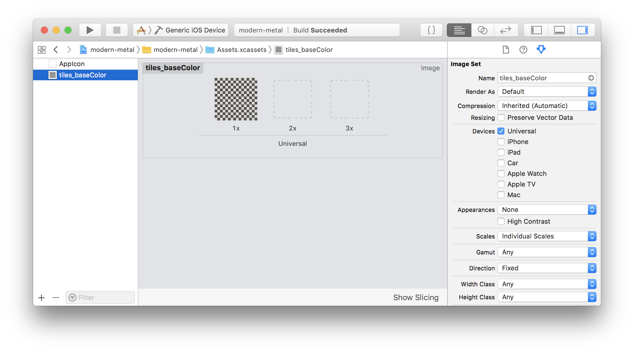
To add images to the project’s asset catalog, select Assets.xcassets in the project navigator and drag images into the side pane. Here, for reference, is what the asset catalog of the sample looks like:

Textures are expensive objects, in terms of how much memory they occupy, and in terms of how long they take to create, so we want to hold references to them rather than creating them frequently. We can add a property to store the base color texture in our renderer:

var baseColorTexture: MTLTexture?

Then we can add the actual texture loading code to the makeResources() method, referencing the image by its name in the asset catalog:

let options: [MTKTextureLoader.Option : Any] = [.generateMipmaps : true, .SRGB : true]
baseColorTexture = try? textureLoader.newTexture(name: "tiles_baseColor", scaleFactor: 1.0, bundle: nil, options: options)

Note that we can supply an options dictionary to affect some aspects of how the texture loader works. One of the options we’re supplying here, .generateMipmaps, is beyond the scope of this article series, but you can read all about mipmapping in Metal here.

Sampler States

Now that we have a texture, we need to tell Metal how to “sample” from it. The details of texture sampling are somewhat beyond the scope of this article, but essentially, we need to decide what happens when more than one texel is mapped to a single fragment (this process is called minification), or when one texel stretches across multiple fragments (called magnification). These choices allow us to make a trade-off between how jagged or blurry our textures appear when there isn’t a one-to-one mapping between pixels and texels.

To communicate these choices to Metal, we create a sampler state. We can use different sampler states to hold different sets of sampling parameters. In the sample project, we’ll only need one sampler for now, so we can add a property for it to the renderer:

let samplerState: MTLSamplerState

To create a sampler state, we fill out a MTLSamplerDescriptor object, then ask the device to create a sampler state for us. We can add a new initializer method for this:

static func buildSamplerState(device: MTLDevice) -> MTLSamplerState {
    let samplerDescriptor = MTLSamplerDescriptor()
    samplerDescriptor.normalizedCoordinates = true
    samplerDescriptor.minFilter = .linear
    samplerDescriptor.magFilter = .linear
    samplerDescriptor.mipFilter = .linear
    return device.makeSamplerState(descriptor: samplerDescriptor)!
}

And as has now become common, call it from the renderer’s initializer:

samplerState = Renderer.buildSamplerState(device: device)

We’ll discuss how to actually use a sampler state object in the next section.

Using Textures in a Fragment Function

Now that we have a texture and a sampler state, we need to actually use them inside our fragment function to determine the base color of each fragment. We can tell Metal which textures and sampler states to use by assigning each of them to an index on the render command encoder:

commandEncoder.setFragmentTexture(baseColorTexture, index: 0)
commandEncoder.setFragmentSamplerState(samplerState, index: 0)

Then, we need to update our fragment function to receive the texture and sampler state and use the sample function on the texture to get the base color:

fragment float4 fragment_main(VertexOut fragmentIn [[stage_in]],
                              texture2d<float, access::sample> baseColorTexture [[texture(0)]],
                              sampler baseColorSampler [[sampler(0)]])
{
    float3 baseColor = baseColorTexture.sample(baseColorSampler, fragmentIn.texCoords).rgb;
    ...
}

Note that the texture parameter is of type texture2d<float, access::sample>, which means that it is a 2-D texture that we intend to sample from, and when we do sample it, we get back a float4 vector containing the RGBA components of the sampled color. Using the access::sample template parameter requires us to have created our texture in such a way that it can be sampled from. Fortunately, MTKTextureLoader takes care of this for us by default.

If we run the sample now, we can see that instead of a solid red teapot, we have a checkered teapot, using the base color texture map to affect the color at every fragment:

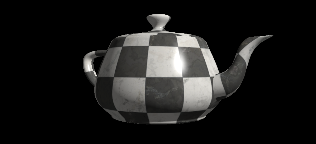
git checkout step2_6 to view the code up to this point.

From One Object to Many

Up until this point, our little world has consisted of a single, central object, but this approach quickly grows limiting. What we really want, in any game or application of reasonable size, is to represent many objects, positioned relative to one another. One popular way of representing objects and their relationships is a scene graph, which is a hierarchy of objects, related by the transforms that move us from the coordinate system of one object to another. Additionally, we might imagine that we want these different objects to have different materials, expressed as different combinations of textures and parameters.

In this section, we will refactor our code to account for many different objects by adding data structures that represent each of the conceptual entities we’ve dealt with so far (lights, materials, and objects), turning them into concrete objects that can be configured and combined into larger scenes.

Refactoring Lights

Previously, we hard-coded the various parameters of our lighting environment (ambient intensity, light direction, and light color) in the shader, but what if we want more than one light in our scene? It makes sense to collect these parameters into their own structure, which we can write (in a new file I’m calling Scene.swift) as:

struct Light {
    var worldPosition = float3(0, 0, 0)
    var color = float3(0, 0, 0)
}

In our shader file, we add a structure that mirrors the Swift struct:

struct Light {
    float3 worldPosition;
    float3 color;
};

Refactoring Vertex Uniforms

Let’s revisit the Uniforms structure. Whereas before, we were only passing uniforms into the vertex function, we’ll now need to pass uniforms into the fragment function as well, so let’s rename the Uniforms struct to VertexUniforms in Renderer.swift:

struct VertexUniforms {
    var viewProjectionMatrix: float4x4
    var modelMatrix: float4x4
    var normalMatrix: float3x3
}

This struct looks pretty much the same in Metal Shading Language:

struct VertexUniforms {
    float4x4 viewProjectionMatrix;
    float4x4 modelMatrix;
    float3x3 normalMatrix;
};

Refactoring Materials

We also need to refactor our representation of materials. The base color of the object naturally comes from the base color texture map, and we can change that each time we draw, but we also need a way to vary the shininess (specular power) of materials, and we’ll also find it convenient to control the color of the specular highlight ⁴. To do this, we create a new Material type. In Swift, it looks like this:

class Material {
    var specularColor = float3(1, 1, 1)
    var specularPower = Float(1)
    var baseColorTexture: MTLTexture?
}

In Metal, we’ll write the specular color and specular power into a new uniforms type, so there is no corresponding Material struct in our shader code.

Introducing Fragment Uniforms

Now we can wrap up these properties into a package of fragment uniforms we’ll pass to our fragment shader. In Swift, it looks like this:

struct FragmentUniforms {
    var cameraWorldPosition = float3(0, 0, 0)
    var ambientLightColor = float3(0, 0, 0)
    var specularColor = float3(1, 1, 1)
    var specularPower = Float(1)
    var light0 = Light()
    var light1 = Light()
    var light2 = Light()
}

Note that because Swift lacks statically-sized arrays, we explicitly add three lights at the end of the struct. If we want to support more lights, we can always add more here.

In Metal, we write the fragment uniforms struct in a similar fashion, except that we define a maximum number of supported lights, and size the lights array according to that count:

#define LightCount 3

struct FragmentUniforms {
    float3 cameraWorldPosition;
    float3 ambientLightColor;
    float3 specularColor;
    float specularPower;
    Light lights[LightCount];
};

That completes the refactoring of uniforms. Now we can get back to the business of writing more flexible shaders that take advantage of these configurable materials and lights.

Lighting Shader Revisited

We need to adapt our fragment function to take the new fragment uniforms, so we add a new parameter that indicates which buffer to read them from (buffer 0), similar to the previously-existing uniforms parameter in the vertex function:

fragment float4 fragment_main(VertexOut fragmentIn [[stage_in]],
                              constant FragmentUniforms &uniforms [[buffer(0)]],
                              texture2d<float, access::sample> baseColorTexture [[texture(0)]],
                              sampler baseColorSampler [[sampler(0)]])

At the top of the new fragment function, we’ll sample the base color as before, and also read the specular color from the fragment uniforms:

float3 baseColor = baseColorTexture.sample(baseColorSampler, fragmentIn.texCoords).rgb;
float3 specularColor = uniforms.specularColor;

Since the world-space normal and world-space viewing direction aren’t dependent on the light location, we can compute them before starting the lighting calculations proper:

float3 N = normalize(fragmentIn.worldNormal.xyz);
float3 V = normalize(uniforms.cameraWorldPosition - fragmentIn.worldPosition.xyz);

Now we can loop over our lights and calculate their individual contributions. The color value of the fragment is the sum of all of the lighting terms contributed by each of the lights:

float3 finalColor(0, 0, 0);
for (int i = 0; i < LightCount; ++i) {
    float3 L = normalize(uniforms.lights[i].worldPosition - fragmentIn.worldPosition.xyz);
    float3 diffuseIntensity = saturate(dot(N, L));
    float3 H = normalize(L + V);
    float specularBase = saturate(dot(N, H));
    float specularIntensity = powr(specularBase, uniforms.specularPower);
    float3 lightColor = uniforms.lights[i].color;
    finalColor += uniforms.ambientLightColor * baseColor +
                  diffuseIntensity * lightColor * baseColor +
                  specularIntensity * lightColor * specularColor;
}

return float4(finalColor, 1);

Feeding the Beast

This completes our refactoring of the lighting shader to account for differing materials and lights. Now we need to patch up the renderer code to feed in all of those new parameters.

Firstly, because we now need to pass in the camera position, we declare it locally (in the draw) method, and use its opposite to compute the view matrix ⁵ :

let cameraWorldPosition = float3(0, 0, 2)
let viewMatrix = float4x4(translationBy: -cameraWorldPosition)

We create an instance of the VertexUniforms struct and pass it into the vertex function:

let viewProjectionMatrix = projectionMatrix * viewMatrix
var vertexUniforms = VertexUniforms(viewProjectionMatrix: viewProjectionMatrix,
                                    modelMatrix: modelMatrix,
                                    normalMatrix: modelMatrix.normalMatrix)
commandEncoder.setVertexBytes(&vertexUniforms, length: MemoryLayout<VertexUniforms>.size, index: 1)

Filling out the fragment uniforms is a bit more involved. We start by declaring a material:

let material = Material()
material.specularPower = 200
material.specularColor = float3(0.8, 0.8, 0.8)

Then, create a few lights with different colors and scatter them around:

let light0 = Light(worldPosition: float3( 2,  2, 2), color: float3(1, 0, 0))
let light1 = Light(worldPosition: float3(-2,  2, 2), color: float3(0, 1, 0))
let light2 = Light(worldPosition: float3( 0, -2, 2), color: float3(0, 0, 1))

Finally, we pack all of those parameters into an instance of FragmentUniforms and tell the command encoder to write it to a buffer at the same index as the one we previously specified in the shader (index 0):

var fragmentUniforms = FragmentUniforms(cameraWorldPosition: cameraWorldPosition,
                                        ambientLightColor: float3(0.1, 0.1, 0.1),
                                        specularColor: material.specularColor,
                                        specularPower: material.specularPower,
                                        light0: light0,
                                        light1: light1,
                                        light2: light2)
commandEncoder.setFragmentBytes(&fragmentUniforms, length: MemoryLayout<FragmentUniforms>.size, index: 0)

What’s the reward for all of this hard work? Well, now our shiny teapot is even shinier, since it’s lit from three different directions:

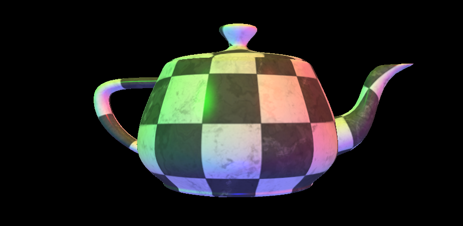
This section laid the groundwork for adding multiple objects to the scene and controlling them independently. In the next section, we’ll actually add multiple objects to the scene and show how to position them relative to one another.

git checkout step2_7 to view the code up to this point.

Nodes and Scene Graphs

In this section we’ll develop an abstraction that will help us do two important things: associate materials and geometry with different objects, and express how objects are positioned and oriented in the world relative to other objects.

A node, in this context, will be an object that has a transform that specifies where it is located and how it is oriented (this is just another 4×4 matrix). A node may also have a reference to a mesh and material which should be used to draw the node. Crucially, nodes also have a reference to their parent and a list of children, which is what defines their place in the hierarchy. A scene graph, then, is a tree of such nodes ⁶.

Node and Scene Types

We’ll start by laying out our basic Node type (this can go in the Scene.swift file, where we’re keeping such things):

class Node {
    var name: String
    weak var parent: Node?
    var children = [Node]()
    var modelMatrix = matrix_identity_float4x4
    var mesh: MTKMesh?
    var material = Material()

    init(name: String) {
        self.name = name
    }
}

We’ll also find it useful to declare a Scene type, which holds the root node (the node that is the ancestor of all other nodes), as well as some lighting parameters. The intention here is to remove as much “teapot-specific” state from the renderer class itself, as we continue to abstract our way toward supporting multiple objects with different materials:

class Scene {
    var rootNode = Node(name: "Root")
    var ambientLightColor = float3(0, 0, 0)
    var lights = [Light]()
}

We can also remove the mesh and material properties from the renderer, replacing them with a reference to a scene, which will (transitively) hold all of that information:

let scene: Scene

Setting a Scene

Since we’re migrating from a hard-coded world to a scene-based approach, we can rename the makeResources method to buildScene, and use it to create our scene instance. Here it is in its entirety:

static func buildScene(device: MTLDevice, vertexDescriptor: MDLVertexDescriptor) -> Scene {
    let bufferAllocator = MTKMeshBufferAllocator(device: device)
    let textureLoader = MTKTextureLoader(device: device)
    let options: [MTKTextureLoader.Option : Any] = [.generateMipmaps : true, .SRGB : true]

    let scene = Scene()

    scene.ambientLightColor = float3(0.01, 0.01, 0.01)
    let light0 = Light(worldPosition: float3( 2,  2, 2), color: float3(1, 0, 0))
    let light1 = Light(worldPosition: float3(-2,  2, 2), color: float3(0, 1, 0))
    let light2 = Light(worldPosition: float3( 0, -2, 2), color: float3(0, 0, 1))
    scene.lights = [ light0, light1, light2 ]

    let teapot = Node(name: "Teapot")

    let modelURL = Bundle.main.url(forResource: "teapot", withExtension: "obj")!
    let asset = MDLAsset(url: modelURL, vertexDescriptor: vertexDescriptor, bufferAllocator: bufferAllocator)
    teapot.mesh = try! MTKMesh.newMeshes(asset: asset, device: device).metalKitMeshes.first
    teapot.material.baseColorTexture = try? textureLoader.newTexture(name: "tiles_baseColor", scaleFactor: 1.0, bundle: nil, options: options)
    teapot.material.specularPower = 200
    teapot.material.specularColor = float3(0.8, 0.8, 0.8)
    scene.rootNode.children.append(teapot)

    return scene
}

First, we create the utility objects we need (the buffer allocator and texture loader). Then we instantiate the scene and configure its lighting environment. Then, we instantiate our teapot node, configuring it with a mesh and various material properties, finally adding it to our scene’s root node and thus adding it to our scene graph.

Now, we can remove the call to makeResources and construct our scene instead:

scene = Renderer.buildScene(device: device, vertexDescriptor: vertexDescriptor)

Updating the Scene

Since we’re updating properties on nodes rather than just calculating transforms on the fly, it makes sense to add an explicit update step, where we do everything time-related.

We can add a few properties to the renderer, which we will update every frame:

var time: Float = 0
var cameraWorldPosition = float3(0, 0, 2)
var viewMatrix = matrix_identity_float4x4
var projectionMatrix = matrix_identity_float4x4

We then write an update method that advances the time variable, updates the view and projection matrices (in case the camera has moved or the view has resized), and updates the transform of the root node to keep the teapot spinning:

func update(_ view: MTKView) {
    time += 1 / Float(view.preferredFramesPerSecond)

    cameraWorldPosition = float3(0, 0, 2)
    viewMatrix = float4x4(translationBy: -cameraWorldPosition)

    let aspectRatio = Float(view.drawableSize.width / view.drawableSize.height)
    projectionMatrix = float4x4(perspectiveProjectionFov: Float.pi / 3, aspectRatio: aspectRatio, nearZ: 0.1, farZ: 100)

    let angle = -time
    scene.rootNode.modelMatrix = float4x4(rotationAbout: float3(0, 1, 0), by: angle) *  float4x4(scaleBy: 1.5)
}

We call this method right at the top of our draw method in order to update every time we render a frame.

Drawing the Scene

Finally, we can put some pixels on the screen. Since we’re still going to wind up with one spinning teapot, this might feel like an anticlimax, but we’ve actually created something very flexible here, and we’ll see the power of the scene graph very shortly.

We can greatly simplify our draw method by extracting the parts of it that relate to setting uniforms and issuing draw calls into a new method. Here’s the revised method:

func draw(in view: MTKView) {
    update(view)

    let commandBuffer = commandQueue.makeCommandBuffer()!
    if let renderPassDescriptor = view.currentRenderPassDescriptor, let drawable = view.currentDrawable {
        let commandEncoder = commandBuffer.makeRenderCommandEncoder(descriptor: renderPassDescriptor)!
        commandEncoder.setFrontFacing(.counterClockwise)
        commandEncoder.setCullMode(.back)
        commandEncoder.setDepthStencilState(depthStencilState)
        commandEncoder.setRenderPipelineState(renderPipeline)
        commandEncoder.setFragmentSamplerState(samplerState, index: 0)
        drawNodeRecursive(scene.rootNode, parentTransform: matrix_identity_float4x4, commandEncoder: commandEncoder)
        commandEncoder.endEncoding()
        commandBuffer.present(drawable)
        commandBuffer.commit()
    }
}

Right in the middle there, you see a call to drawNodeRecursive, which is the real workhorse of the render step. First, let’s take a look at its skeleton:

func drawNodeRecursive(_ node: Node, parentTransform: float4x4, commandEncoder: MTLRenderCommandEncoder) {
    let modelMatrix = parentTransform * node.modelMatrix
    // ...
    for child in node.children {
        drawNodeRecursive(child, parentTransform: modelMatrix, commandEncoder: commandEncoder)
    }
}

At the top, we compute a local model matrix, which is the product of the parentTransform parameter and the model matrix of the current node. This combined model matrix will move us to world space through the model space of our parent node. At the end of the method, we pass this same transform recursively into this method so that the children of this node are additionally transformed by the transform of this node. By descending the scene graph (tree) and transforming each node by the product of its ancestors’ transforms, we effectively position those objects relative to one another.

The interior of this method is very similar to our previous draw method: build the uniforms structs, set the texture, and draw. Here’s drawNodeRecursive in its entirety:

    func drawNodeRecursive(_ node: Node, parentTransform: float4x4, commandEncoder: MTLRenderCommandEncoder) {
        let modelMatrix = parentTransform * node.modelMatrix

        if let mesh = node.mesh, let baseColorTexture = node.material.baseColorTexture {
            let viewProjectionMatrix = projectionMatrix * viewMatrix
            var vertexUniforms = VertexUniforms(viewProjectionMatrix: viewProjectionMatrix,
                                                modelMatrix: modelMatrix,
                                                normalMatrix: modelMatrix.normalMatrix)
            commandEncoder.setVertexBytes(&vertexUniforms, length: MemoryLayout<VertexUniforms>.size, index: 1)

            var fragmentUniforms = FragmentUniforms(cameraWorldPosition: cameraWorldPosition,
                                                    ambientLightColor: scene.ambientLightColor,
                                                    specularColor: node.material.specularColor,
                                                    specularPower: node.material.specularPower,
                                                    light0: scene.lights[0],
                                                    light1: scene.lights[1],
                                                    light2: scene.lights[2])
            commandEncoder.setFragmentBytes(&fragmentUniforms, length: MemoryLayout<FragmentUniforms>.size, index: 0)

            commandEncoder.setFragmentTexture(baseColorTexture, index: 0)

            let vertexBuffer = mesh.vertexBuffers.first!
            commandEncoder.setVertexBuffer(vertexBuffer.buffer, offset: vertexBuffer.offset, index: 0)

            for submesh in mesh.submeshes {
                let indexBuffer = submesh.indexBuffer
                commandEncoder.drawIndexedPrimitives(type: submesh.primitiveType,
                                                     indexCount: submesh.indexCount,
                                                     indexType: submesh.indexType,
                                                     indexBuffer: indexBuffer.buffer,
                                                     indexBufferOffset: indexBuffer.offset)
            }
        }

        for child in node.children {
            drawNodeRecursive(child, parentTransform: modelMatrix, commandEncoder: commandEncoder)
        }
    }

Finding Nodes by Name

Each node in the scene graph has a name. If these names are unique, we can use them to locate a node anywhere in the scene graph by name. Adding this functionality to our Scene and Node classes is another straightforward exercise in recursion.

First, let’s implement nodeNamedRecursive(:) in the Node class. The gist of the algorithm is this: for each child of the current node, if the child has the name we’re looking for, return that child. Otherwise, ask each child in turn whether it has a descendant with the name and return the first match. If no match is found, return nil. Here it is in Swift:

func nodeNamedRecursive(_ name: String) -> Node? {
    for node in children {
        if node.name == name {
            return node
        } else if let matchingGrandchild = node.nodeNamedRecursive(name) {
            return matchingGrandchild
        }
    }
    return nil
}

We implement the nodeNamed method in the Scene class in terms of the nodeNamedRecursive method:

func nodeNamed(_ name: String) -> Node? {
    if rootNode.name == name {
        return rootNode
    } else {
        return rootNode.nodeNamedRecursive(name)
    }
}

git checkout step2_8 to view the code up to this point.

Creating a More Interesting Scene

“Okay, enough with the teapots,” I hear you saying. Let’s create a scene with some action. I’m a big fan of Kennan Crane’s public domain models, so we’ll borrow a couple of them.

Meet Bob and Blub

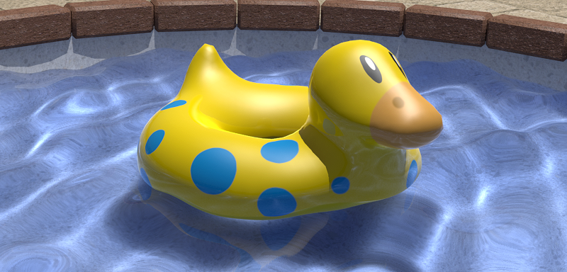
Bob is a model of an inflatable duck float. We’ll load it in pretty much the same way we loaded the teapot model, and also load its accompanying texture. We combine the mesh and texture in a new node named “Bob” and add it to the root of our scene like so:

let bob = Node(name: "Bob")
let bobMaterial = Material()
let bobBaseColorTexture = try? textureLoader.newTexture(name: "bob_baseColor",
                                                        scaleFactor: 1.0,
                                                        bundle: nil,
                                                        options: options)
bobMaterial.baseColorTexture = bobBaseColorTexture
bobMaterial.specularPower = 100
bobMaterial.specularColor = float3(0.8, 0.8, 0.8)
bob.material = bobMaterial

let bobURL = Bundle.main.url(forResource: "bob", withExtension: "obj")!
let bobAsset = MDLAsset(url: bobURL, vertexDescriptor: vertexDescriptor, bufferAllocator: bufferAllocator)
bob.mesh = try! MTKMesh.newMeshes(asset: bobAsset, device: device).metalKitMeshes.first!

scene.rootNode.children.append(bob)

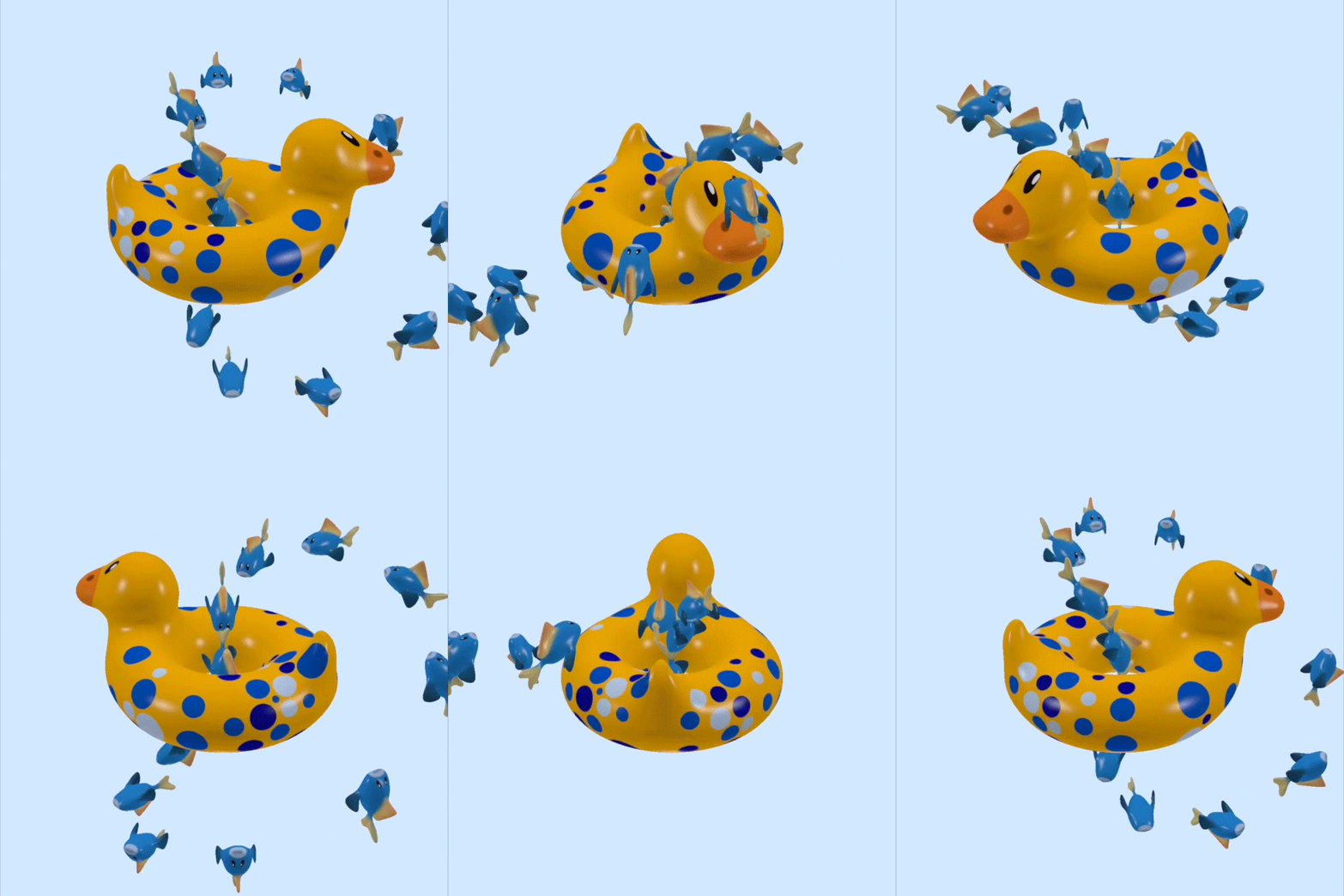
Let’s give Bob some friends. Another Keenan Crane model, Blub, is a blue fish.

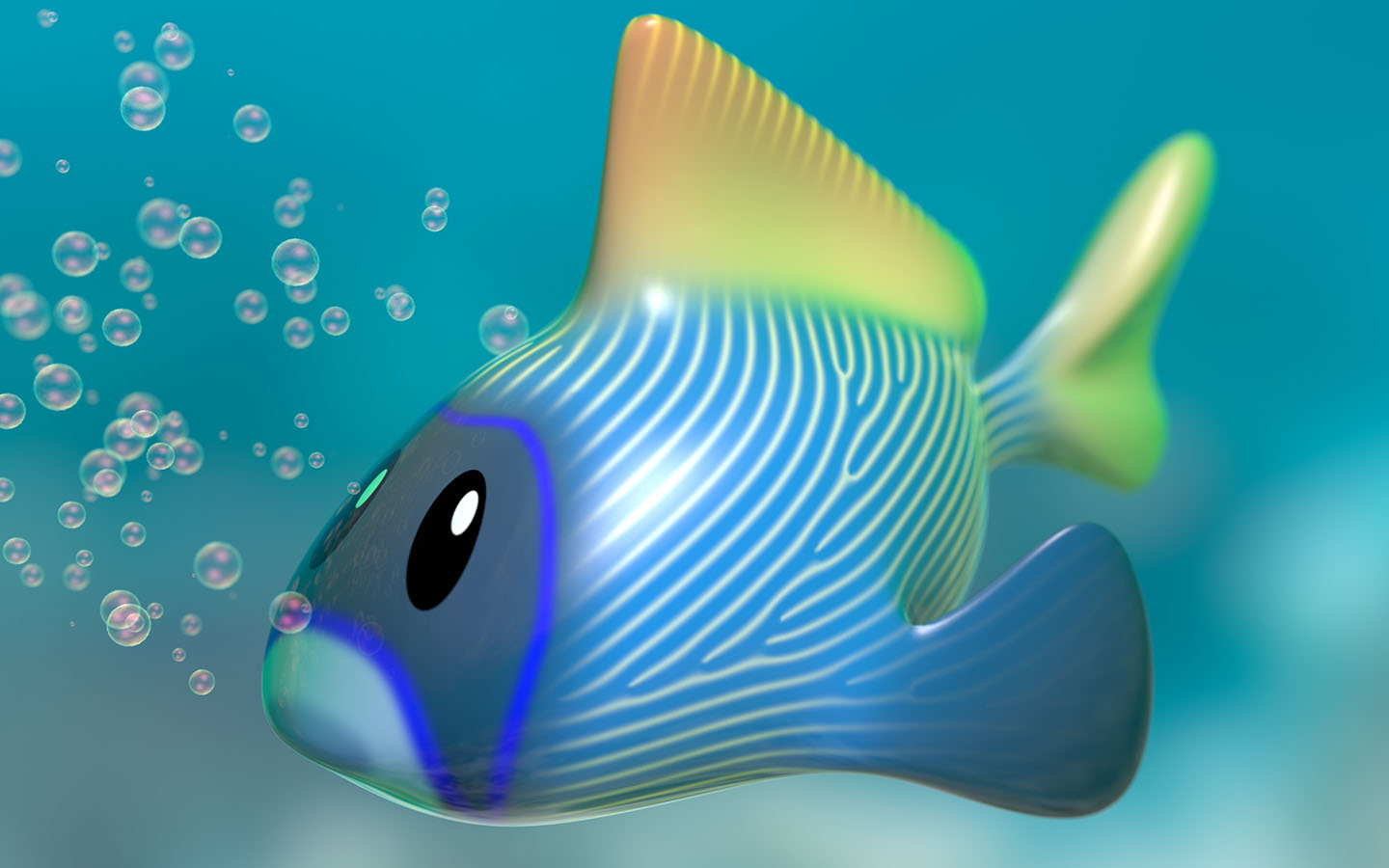
We’ll create several Blubs and add them to Bob so they can do some aquabatics together. We load Blub in exactly the same way we loaded Bob, but this time we create several nodes in a loop and give each one a unique name so we can reference them later when animating (“Blub 1”, “Blub 2”, etc.):

let blubMaterial = Material()
let blubBaseColorTexture = try? textureLoader.newTexture(name: "blub_baseColor",
                                                         scaleFactor: 1.0,
                                                         bundle: nil,
                                                         options: options)
blubMaterial.baseColorTexture = blubBaseColorTexture
blubMaterial.specularPower = 40
blubMaterial.specularColor = float3(0.8, 0.8, 0.8)

let blubURL = Bundle.main.url(forResource: "blub", withExtension: "obj")!
let blubAsset = MDLAsset(url: blubURL, vertexDescriptor: vertexDescriptor, bufferAllocator: bufferAllocator)
let blubMesh = try! MTKMesh.newMeshes(asset: blubAsset, device: device).metalKitMeshes.first!

for i in 1...fishCount {
    let blub = Node(name: "Blub \(i)")
    blub.material = blubMaterial
    blub.mesh = blubMesh
    bob.children.append(blub)
}

Animating Bob and Blub

It doesn’t make much sense to have a pool float named Bob that doesn’t actually bob. Let’s add some code to the update method to displace Bob by a small amount vertically according to a sine wave, which will make him appear like he’s bobbing up and down on gently lapping water:

if let bob = scene.nodeNamed("Bob") {
    bob.modelMatrix = float4x4(translationBy: float3(0, 0.015 * sin(time * 5), 0))
}

Note that we used the nodeNamed method to look Bob up by name. We could also have kept a reference to the Bob node when we created it.

Now let’s animate our Blubs. Their behavior is somewhat more complex: each fish’s transform is composed of a number of basic transform matrices that scale, translate, and rotate each fish into the correct size, position, and orientation:

let blubBaseTransform = float4x4(rotationAbout: float3(0, 0, 1), by: -.pi / 2) *
                        float4x4(scaleBy: 0.25) *
                        float4x4(rotationAbout: float3(0, 1, 0), by: -.pi / 2)

let fishCount = Renderer.fishCount
for i in 1...fishCount {
    if let blub = scene.nodeNamed("Blub \(i)") {
        let pivotPosition = float3(0.4, 0, 0)
        let rotationOffset = float3(0.4, 0, 0)
        let rotationSpeed = Float(0.3)
        let rotationAngle = 2 * Float.pi * Float(rotationSpeed * time) + (2 * Float.pi / Float(fishCount) * Float(i - 1))
        let horizontalAngle = 2 * .pi / Float(fishCount) * Float(i - 1)
        blub.modelMatrix = float4x4(rotationAbout: float3(0, 1, 0), by: horizontalAngle) *
                           float4x4(translationBy: rotationOffset) *
                           float4x4(rotationAbout: float3(0, 0, 1), by: rotationAngle) *
                           float4x4(translationBy: pivotPosition) *
                           blubBaseTransform
    }
}

And here’s the result, a rather engrossing display of marine talent, if I may say so:

git checkout step2_9 to view the final version of the code for this article.

In Closing

We covered a ton of ground in this article. From basic materials and lighting, to texturing, all the way to basics of scene graphs. I hope you’ve enjoyed following along! Feel free to comment below with any questions.